Getting started with oda

oda

2026-06-15

oda is a pure-R implementation of the MegaODA / CTA classification engine. It provides three main tools:

• oda_fit() - Optimal Data Analysis (ODA): univariate binary or multiclass classification with a single attribute.
• cta_fit() - Classification Tree Analysis (CTA): recursive ODA-node trees with ENUMERATE, LOO STABLE, and MINDENOM endpoint constraints.
• Translation and graphics - endpoint staging, propensity weights, tree plots, and NOVOmetric bootstrap CIs via cta_staging_table(), cta_propensity_weights(), novo_boot_ci(), plot.cta_tree(), and the ggplot2 renderers plot_cta_tree() / plot_lort_tree() (requires ggplot2).

Binary ODA

oda_fit() finds the single cutpoint that maximises Mean PAC (percentage of accurate classifications, averaged across classes with inverse-frequency weighting when priors_on = TRUE). ESS (Effect Strength for Sensitivity) measures how far Mean PAC exceeds the chance benchmark of 50%.

library(oda)

x <- c(1, 2, 3, 4, 5, 6, 7, 8)
y <- c(0L, 0L, 0L, 0L, 1L, 1L, 1L, 1L)

fit <- oda_fit(x, y, mcarlo = FALSE)
print(fit)
#> 
#> ODA (binary)  attr_type=ordered  priors=TRUE  n=8
#> 
#> Rule: <= 4.5 --> 0   |   > 4.5 --> 1
#> 
#>   CLASS       n     PAC
#>       0       4  100.0%
#>       1       4  100.0%
#> 
#>   Mean PAC: 100.00%   ESS: 100.00%

The fitted rule, per-class PAC, Mean PAC, and ESS are available directly:

fit$rule$cut_value    # cutpoint
#> [1] 4.5
fit$rule$direction    # which side maps to class 1
#> [1] "0->1"
fit$ess               # ESS (%)
#> [1] 100

Classification Tree Analysis

cta_fit() grows a binary classification tree in which each split node is an ODA model. mindenom sets the minimum leaf size; mc_iter controls the Monte Carlo permutation test used to screen candidate splits; loo = "stable" keeps only splits whose leave-one-out ESS matches the training ESS.

The example below uses a small synthetic dataset. For publication analyses use at least mc_iter = 5000L.

X <- data.frame(
  x1 = c(1, 2, 3, 4, 5, 6, 7, 8),
  x2 = c(0L, 0L, 1L, 0L, 1L, 1L, 0L, 1L)
)
y <- c(1L, 1L, 1L, 1L, 2L, 2L, 2L, 2L)

tree <- cta_fit(X, y,
  priors_on  = TRUE,
  mindenom   = 2L,
  mc_iter    = 500L,
  mc_seed    = 42L,
  loo        = "off",
  attr_names = c("x1", "x2")
)
print(tree)
#> 
#> CTA Tree  alpha_split=0.050  mindenom=2  prune=1.000  max_depth=10  loo=off
#> 
#> ATTRIBUTE      NODE  LEV    OBS       p      ESS     WESS      LOO  MODEL
#> ---------------------------------------------------------------------------------- 
#> x1                1    1      8   0.026  100.00%  100.00%      OFF  <=4.5-->0; >4.5-->1
#>   Node-local split confusion (this rule only, observations at this node)
#>                    0      1 
#>              -------------- 
#>        0  |       4      0 | 100.00%
#>        1  |       0      4 | 100.00%
#>              -------------- 
#>       NP  |       4      4
#> 
#> Nodes: 3 total  (1 split  2 leaf)
#> 
#> Terminal endpoints (*):
#> * endpoint 1  node 2:  path=x1<=4.5  n=4  counts=[0:4 1:0]  predicted=0  target_prop=0.0%
#> * endpoint 2  node 3:  path=x1>4.5  n=4  counts=[0:0 1:4]  predicted=1  target_prop=100.0%
#> ESS: 100.00%  D: 0.0000  strata: 2  min_denom: 4

plot(tree)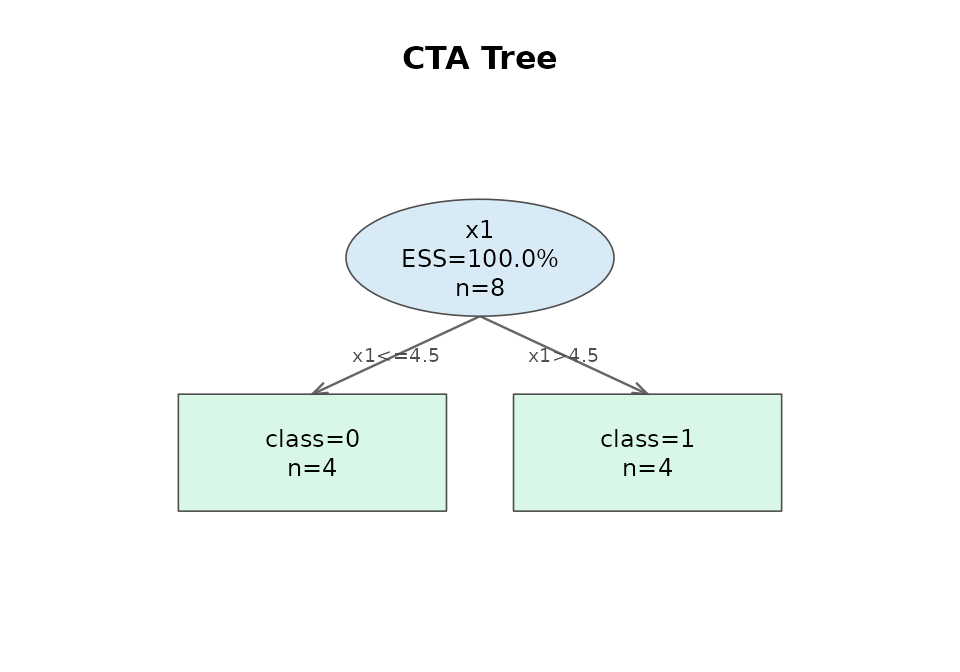

Further reading

The public pkgdown article series currently focuses on stable, publication-ready workflows:

Article	Content
ODA basics	oda_fit() in depth: rule, PAC, ESS, LOO
Directional ODA	Directional binary ODA and fixed/identity-map categorical examples
Multiclass ODA	C >= 3 class variables; PAC per class; K-class chance benchmark
CTA basics	cta_fit(): MINDENOM, LOO STABLE, ENUMERATE, pruning
CTA graphics	cta_plot_data() data contract; plot.cta_tree() and plot_cta_tree() renderers
NOVOboot CI	novo_boot_ci(): fixed-confusion NOVOmetric bootstrap for binary 2 x 2 confusion tables

The example-driven package vignettes are available after installing with build_vignettes = TRUE and running browseVignettes("oda"):

Vignette	Content
Binary ODA: Migraine Attacks	Binary ordered ODA example
Binary Ordered Directional ODA: The Refugee Act	Directional ordered ODA example
Binary Categorical ODA: Gully Erosion	Nondirectional MegaODA parity run for the gully example
Multiclass Categorical ODA: Protein Type	Nondirectional MegaODA parity run for the protein example

Note: Some longer-form draft articles, including the full practitioner guide, validation tiers, CTA translation, MDSA family, and myeloma CTA walkthrough, are intentionally withheld from the public site until their examples and artifacts are finalized.