CTA Tree Diagrams (base-R and ggplot2)

oda provides two levels of CTA tree visualisation:

• Base-R renderers (plot.cta_tree, plot.cta_ort): no external dependencies; structural diagram via base graphics.
• ggplot2 renderers (plot_cta_tree, plot_lort_tree): requires the ggplot2 package; richer control over colour and layout.

Both share the same data contract: cta_plot_data() (for CTA trees) and ort_plot_data() (for LORT trees) produce renderer-independent plot-data objects. You can pass either the fit object directly or a pre-computed plot-data object to any renderer.

cta_plot_data(): the renderer-independent data contract

cta_plot_data() extracts node/edge geometry, split rules, class counts, and terminal predictions from a fitted cta_tree object. The result is a self-contained plot-data object usable by any renderer.

library(oda)

set.seed(1L)
n <- 60L
X <- data.frame(
  x1 = c(rnorm(30, mean = 2), rnorm(30, mean = 5)),
  x2 = c(rnorm(30, mean = 1), rnorm(30, mean = 3))
)
y <- c(rep(1L, 30), rep(2L, 30))

tree <- cta_fit(X, y,
  mindenom   = 12L,
  mc_iter    = 300L,
  mc_seed    = 42L,
  loo        = "off",
  attr_names = c("x1", "x2")
)

pd <- cta_plot_data(tree)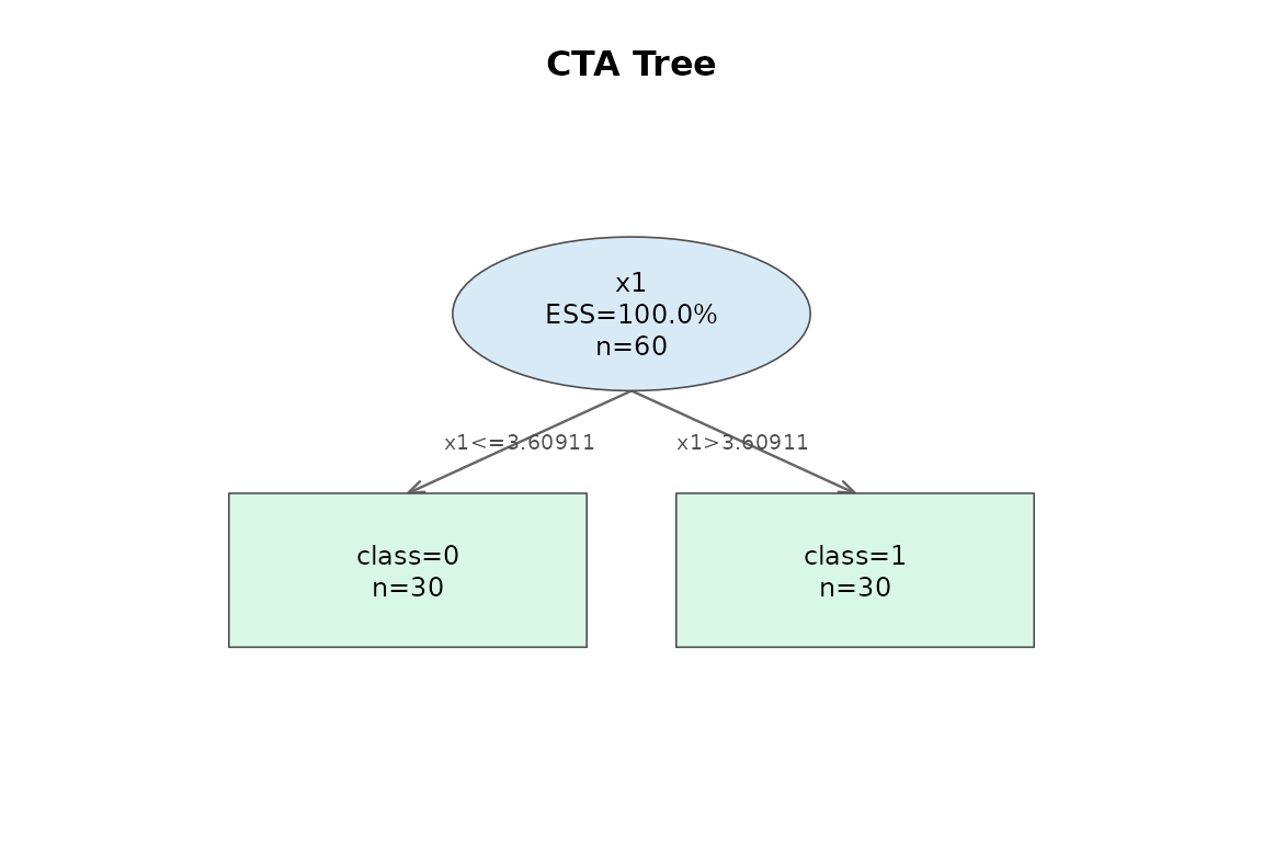

plot.cta_tree(): native base-R renderer

plot(tree)

Graphics v3: ggplot2 renderers

plot_cta_tree() requires ggplot2 (in Suggests). The function accepts either the fit object or pre-computed plot-data. color_by controls terminal-node fill:

• "none" (default): white fill - B/W, publication-ready with no legend.
• "prediction": discrete fill by predicted class.
• "target_rate": continuous gradient by target-class proportion.

plot_cta_tree(pd, color_by = "prediction")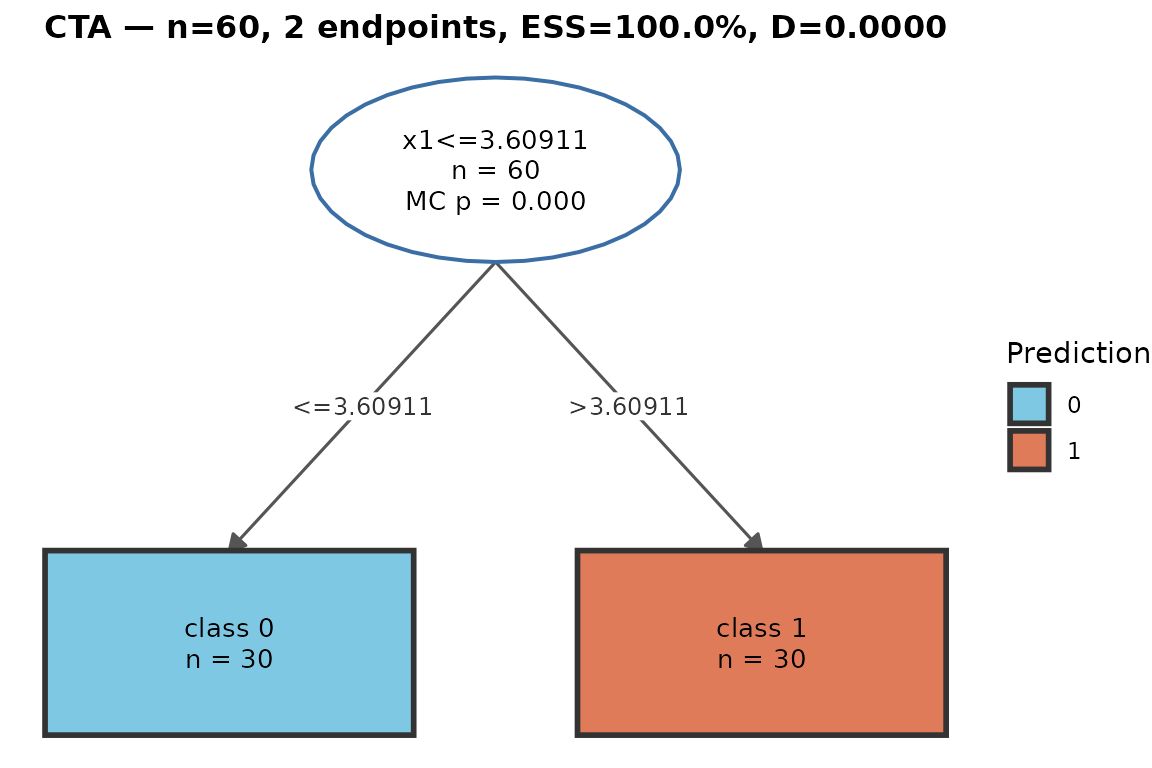

# target_rate: gradient showing proportion of class 1 per node
plot_cta_tree(pd, color_by = "target_rate", target_class = 1L)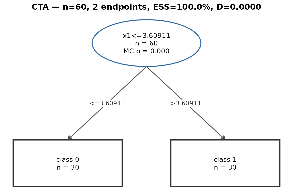

Saving to file:

if (requireNamespace("ggplot2", quietly = TRUE)) {
  p <- plot_cta_tree(pd)
  ggplot2::ggsave("cta_tree.png", p, width = 8, height = 5, dpi = 150)
}

Endpoint label content

Each leaf label shows the predicted class, total n at the endpoint, and (when target_class is set) the raw target-class count and proportion. These values come directly from the per-leaf class_counts_raw stored at fit time - no recomputation occurs inside the renderer.

Endpoint colouring encodes relative target-class proportion within this tree only. It does not imply prevalence, risk, or any external reference standard.

LORT trees

LORT (Locally Optimal Recursive Trees) are displayed by indexed sub-tree inspection. plot_lort_tree(lort, index = k) renders the CTA sub-tree at LORT node k. show_all = TRUE returns a named list of ggplot objects.

lort <- lort_fit(X, y, mc_iter = 300L, mc_seed = 42L, min_n = 12L)
# Root sub-tree (default index = 1)
plot_lort_tree(lort, color_by = "prediction")
# All sub-trees as a named list
all_plots <- plot_lort_tree(lort, show_all = TRUE)

Further reading

• docs/GRAPHICS_V3.md - full v3 function reference, examples, and ggsave usage
• articles/cta-basics - CTA fitting and predict.cta_tree()